Brain decoding with GCN¶

Brain graph representation¶

Graph signal processing is a new tool to model brain organization and function. The brain is composed of several Region of Interests(ROIs). Brain graphs provide an efficient way for modeling the human brain connectome, by associating nodes to the brain regions, and defining edges via anatomical or functional connections. These ROIs are connected to some regions of interests with the highest connectivity.

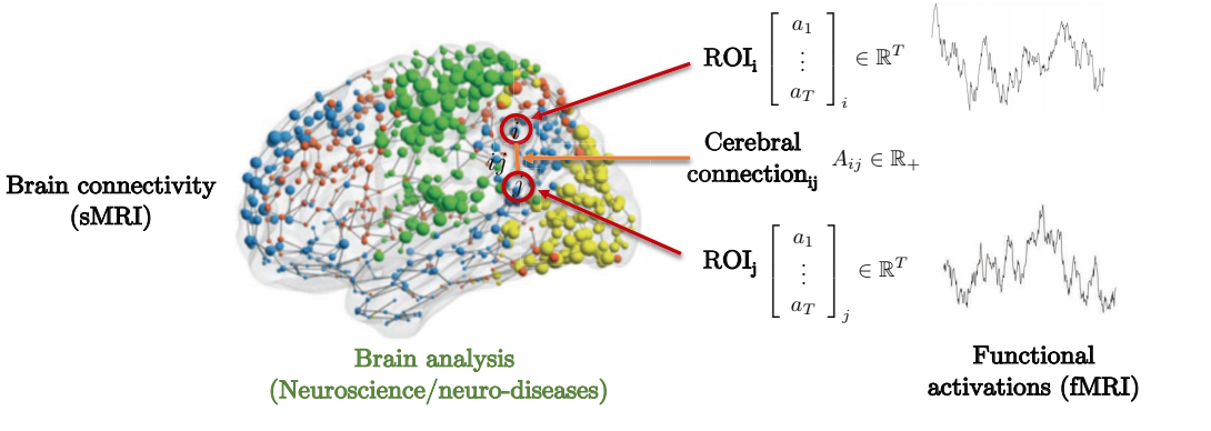
Representation of Brain connectivity by graph theory. Image source:https://atcold.github.io/pytorch-Deep-Learning/en/week13/13-1/

Graph Convolution Network (GCN)¶

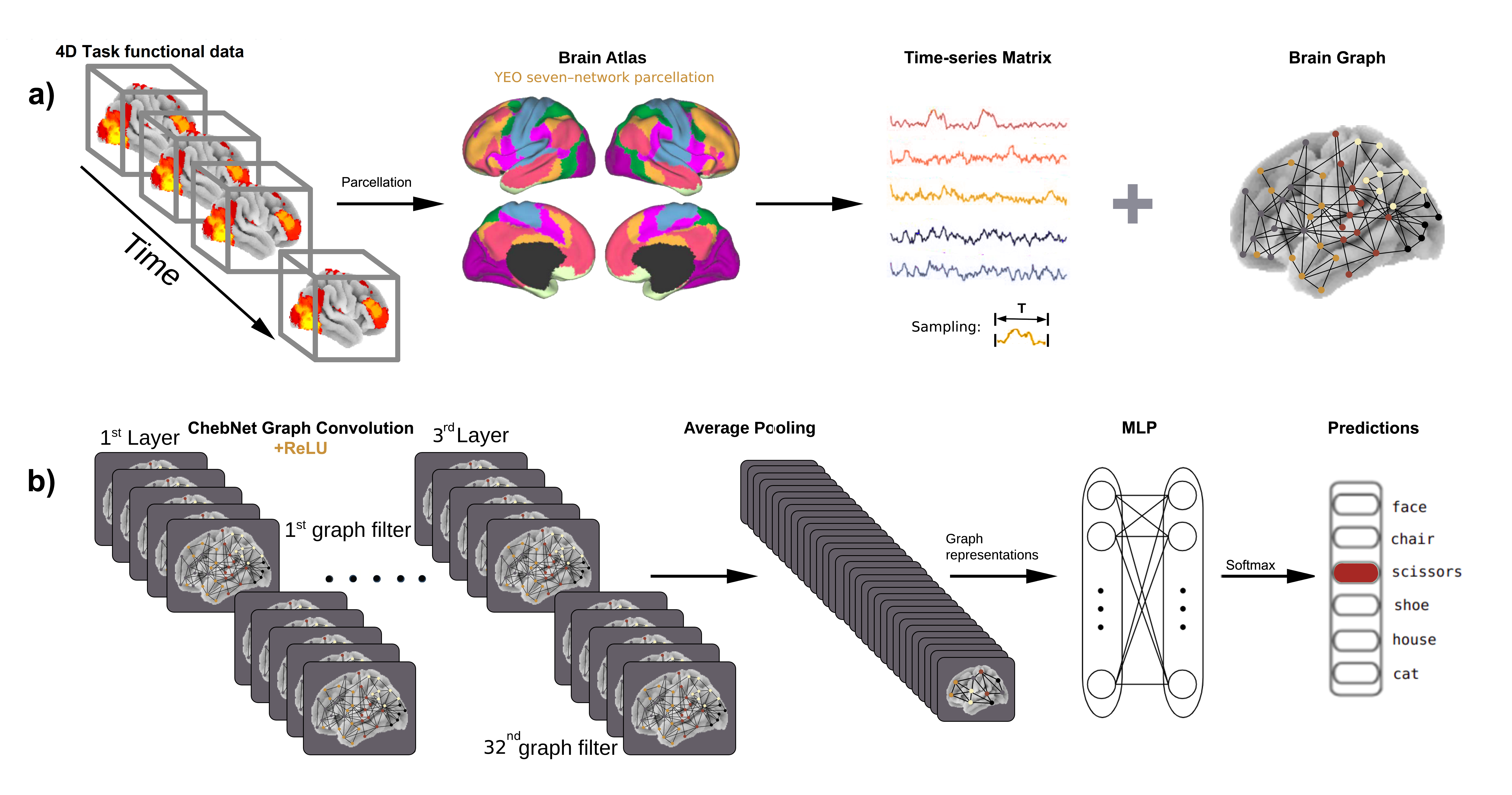
Schematic view of brain decoding using graph convolution network. Model is adapted from Zhang and colleagues (2021). a) Bold time series are used to construct the brain graph by associating nodes to predefined brain regions (parcels) and indicating edges between each pair of brain regions based on the strength of their connections. Then, both brain graph and time-series matrix are imported into the graph convolutional network b) The decoding model consists of three graph convolutional layers with 32 ChebNet graph filters at each layer, followed by a global average pooling layer, two fully connected layers (MLP, consisting of 256-128 units) and softmax function. This pipeline generates task-specific representations of recorded brain activities and predicts the corresponding cognitive states.

Getting the data¶

We are going to download the dataset from Haxby and colleagues (2001) [HGF+01]. You can check An overview of the Haxby dataset section for more details on that dataset. Here we are going to quickly download it, and prepare it for machine learning applications with a set of predictive variable, the brain time series, and a dependent variable, the annotation on cognition.

import os
import warnings
warnings.filterwarnings(action='once')
from nilearn.input_data import NiftiMasker

from nilearn import datasets

# We are fetching the data for subject 4
data_dir = os.path.join('..', 'data')
sub_no = 4
haxby_dataset = datasets.fetch_haxby(subjects=[sub_no], fetch_stimuli=True, data_dir=data_dir)
func_file = haxby_dataset.func[0]

# Standardizing
mask_vt_file = haxby_dataset.mask_vt[0]
masker = NiftiMasker(mask_img=mask_vt_file, standardize=True)

# cognitive annotations
import pandas as pd
behavioral = pd.read_csv(haxby_dataset.session_target[0], delimiter=' ')
X = masker.fit_transform(func_file)
y = behavioral['labels']

/opt/hostedtoolcache/Python/3.8.16/x64/lib/python3.8/site-packages/nilearn/datasets/func.py:20: DeprecationWarning: Please use `MatReadError` from the `scipy.io.matlab` namespace, the `scipy.io.matlab.miobase` namespace is deprecated.
  from scipy.io.matlab.miobase import MatReadError
/opt/hostedtoolcache/Python/3.8.16/x64/lib/python3.8/site-packages/nilearn/datasets/__init__.py:93: FutureWarning: Fetchers from the nilearn.datasets module will be updated in version 0.9 to return python strings instead of bytes and Pandas dataframes instead of Numpy arrays.
  warn("Fetchers from the nilearn.datasets module will be "

Dataset created in ../data/haxby2001

Downloading data from https://www.nitrc.org/frs/download.php/7868/mask.nii.gz ...

 ...done. (0 seconds, 0 min)

Downloading data from http://data.pymvpa.org/datasets/haxby2001/MD5SUMS ...

 ...done. (0 seconds, 0 min)

Downloading data from http://data.pymvpa.org/datasets/haxby2001/subj4-2010.01.14.tar.gz ...

Downloaded 38535168 of 329954386 bytes (11.7%,    7.6s remaining)

Downloaded 92831744 of 329954386 bytes (28.1%,    5.2s remaining)

Downloaded 136232960 of 329954386 bytes (41.3%,    4.3s remaining)

Downloaded 179044352 of 329954386 bytes (54.3%,    3.4s remaining)

Downloaded 226803712 of 329954386 bytes (68.7%,    2.3s remaining)

Downloaded 283230208 of 329954386 bytes (85.8%,    1.0s remaining)

 ...done. (7 seconds, 0 min)

Extracting data from ../data/haxby2001/622d4f5d4b8f14a567901606c924e90d/subj4-2010.01.14.tar.gz...

.. done.

Downloading data from http://data.pymvpa.org/datasets/haxby2001/stimuli-2010.01.14.tar.gz ...

 ...done. (1 seconds, 0 min)
Extracting data from ../data/haxby2001/5cd78c74b711572c7f41a5bddb69abca/stimuli-2010.01.14.tar.gz..... done.

Let’s check the shape of X and y and the cognitive annotations of this data sample.

categories = y.unique()
print(categories)
print('y:', y.shape)
print('X:', X.shape)

['rest' 'face' 'chair' 'scissors' 'shoe' 'scrambledpix' 'house' 'cat'
 'bottle']
y: (1452,)
X: (1452, 675)

So we have 1452 time points in the imaging data, and for each time point we have recordings of fMRI activity across 675 brain regions.

Create brain graph for GCN¶

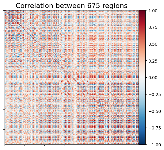
A key component of GCN is brain graph. Brain graph provides a network representation of brain organization by associating nodes to brain regions and defining edges via anatomical or functional connections. After generating time series, we will firstly use the nilearn function to geneate a correlation based functional connectome.

Basic of graph laplacian and graph convolutional networks.

To explore the basics of graph laplacian and graph convolutional networks and how to apply these tools to neuroimging data check the tutorial from MAIN 2019 conference presented by Dr. Zhang.

GCN_tutorial_slides:
Github repo: Binder projects:

import warnings
warnings.filterwarnings(action='once')

import nilearn.connectome

# Estimating connectomes and save for pytorch to load
corr_measure = nilearn.connectome.ConnectivityMeasure(kind="correlation")
conn = corr_measure.fit_transform([X])[0]

n_regions_extracted = X.shape[-1]
title = 'Correlation between %d regions' % n_regions_extracted

print('Correlation matrix shape:',conn.shape)

# First plot the matrix
from nilearn import plotting
display = plotting.plot_matrix(conn, vmax=1, vmin=-1,
                               colorbar=True, title=title)

Correlation matrix shape: (675, 675)

The next step is to construct the brain graph for GCN.

k-Nearest Neighbours(KNN) graph for the group average connectome will be built based on the connectivity-matrix.

Each node is only connected to k conn = corr_measure.fit_transform([X])[0] other neighbouring nodes. For the purpose of demostration, we constrain the graph to from clusters with 8 neighbouring nodes with the strongest connectivity.

For more details you please check out src/graph_construction.py script.

import sys
sys.path.append('../src')
from graph_construction import make_group_graph

# make a graph for the subject
graph = make_group_graph([conn], self_loops=False, k=8, symmetric=True)

Preparing the dataset for model training¶

The trials for different object categories are scattered in the experiment. Firstly we will concatenated the volumes of the same category together.

# generate data
import pandas as pd
import numpy as np

# cancatenate the same type of trials
concat_bold = {}
for label in categories:
    cur_label_index = y.index[y == label].tolist()
    curr_bold_seg = X[cur_label_index]    
    concat_bold[label] = curr_bold_seg

We split the data by the time window size that we wish to use to caputre the temporal dynamic. Different lengths for our input data can be selected. In this example we will continue with window_length = 1, which means each input file will have a length equal to just one Repetition Time (TR). The splitted timeseries are saved as individual files (in the format of <category>_seg_<serialnumber>.npy), the file names and the associated label are stored in the same directory, under a file named label.csv.

# split the data by time window size and save to file
window_length = 1
dic_labels = {name: i for i, name in enumerate(categories)}

# set output paths
split_path = os.path.join(data_dir, 'haxby_split_win/')
if not os.path.exists(split_path):
    os.makedirs(split_path)
out_file = os.path.join(split_path, '{}_{:04d}.npy')
out_csv = os.path.join(split_path, 'labels.csv')

label_df = pd.DataFrame(columns=['label', 'filename'])
for label, ts_data in concat_bold.items():
    ts_duration = len(ts_data)
    ts_filename = f"{label}_seg"
    valid_label = dic_labels[label]

    # Split the timeseries
    rem = ts_duration % window_length
    n_splits = int(np.floor(ts_duration / window_length))

    ts_data = ts_data[:(ts_duration - rem), :]   

    for j, split_ts in enumerate(np.split(ts_data, n_splits)):
        ts_output_file_name = out_file.format(ts_filename, j)

        split_ts = np.swapaxes(split_ts, 0, 1)
        np.save(ts_output_file_name, split_ts)

        curr_label = {'label': valid_label, 'filename': os.path.basename(ts_output_file_name)}
        label_df = label_df.append(curr_label, ignore_index=True)
        
label_df.to_csv(out_csv, index=False)  

Now we use a customised pytorch dataset generator class TimeWindowsDataset to split the data into training, validation, and testing sets for model selection.

The dataset generator defaults isolates 20% of the data as the validation set, and 10% as testing set. For more details of customising a dataset, please see src/gcn_windows_dataset.py and the official pytorch documentation.

# split dataset
from gcn_windows_dataset import TimeWindowsDataset

random_seed = 0

train_dataset = TimeWindowsDataset(
    data_dir=split_path, 
    partition="train", 
    random_seed=random_seed, 
    pin_memory=True, 
    normalize=True,
    shuffle=True)

valid_dataset = TimeWindowsDataset(
    data_dir=split_path, 
    partition="valid", 
    random_seed=random_seed, 
    pin_memory=True, 
    normalize=True,
    shuffle=True)

test_dataset = TimeWindowsDataset(
    data_dir=split_path, 
    partition="test", 
    random_seed=random_seed, 
    pin_memory=True, 
    normalize=True,
    shuffle=True)

print("train dataset: {}".format(train_dataset))
print("valid dataset: {}".format(valid_dataset))
print("test dataset: {}".format(test_dataset))

train dataset: 1016*(torch.Size([675, 1]), ())
valid dataset: 290*(torch.Size([675, 1]), ())
test dataset: 146*(torch.Size([675, 1]), ())

Once the datasets are created, we can use the pytorch data loader to iterate through the data during the model selection process. The batch size defines the number of samples that will be propagated through the neural network. We are separating the dataset into 10 time windows per batch.

import torch
from torch.utils.data import DataLoader

batch_size = 10

torch.manual_seed(random_seed)
train_generator = DataLoader(train_dataset, batch_size=batch_size, shuffle=True)
valid_generator = DataLoader(valid_dataset, batch_size=batch_size, shuffle=True)
test_generator = DataLoader(test_dataset, batch_size=batch_size, shuffle=True)
train_features, train_labels = next(iter(train_generator))
print(f"Feature batch shape: {train_features.size()}; mean {torch.mean(train_features)}")
print(f"Labels batch shape: {train_labels.size()}; mean {torch.mean(torch.Tensor.float(train_labels))}")

Feature batch shape: torch.Size([10, 675, 1]); mean -5.08626296635839e-09
Labels batch shape: torch.Size([10]); mean 2.5999999046325684

Generating a GCN model¶

We have created a GCN of the following property:

3 graph convolutional layers
32 graph filters at each layer
followed by a global average pooling layer
2 fully connected layers

from gcn_model import GCN

gcn = GCN(graph.edge_index, 
          graph.edge_attr, 
          n_roi=X.shape[1],
          batch_size=batch_size,
          n_timepoints=window_length, 
          n_classes=len(categories))
gcn

GCN(
  (conv1): ChebConv(1, 32, K=2, normalization=sym)
  (conv2): ChebConv(32, 32, K=2, normalization=sym)
  (conv3): ChebConv(32, 10, K=2, normalization=sym)
  (fc1): Linear(in_features=6750, out_features=256, bias=True)
  (fc2): Linear(in_features=256, out_features=128, bias=True)
  (fc3): Linear(in_features=128, out_features=9, bias=True)
  (dropout): Dropout(p=0.2, inplace=False)
)

Train and evaluating the model¶

We will use a procedure called backpropagation to train the model. When we training the model with the first batch of data, the accuarcy and loss will be pretty poor. Backpropagation is an algorithm to update the model based on the rate of loss. Iterating through each batch, the model will be updated and reduce the loss.

Function training_loop performs backpropagation through pytorch. One can use their own choice of optimizer for backpropagation and estimator for loss.

After one round of training, we use the validation dataset to calculate the average accuracy and loss with function valid_test_loop. These metrics will serve as the reference for model performance of this round of training.

def train_loop(dataloader, model, loss_fn, optimizer):
    size = len(dataloader.dataset)    

    for batch, (X, y) in enumerate(dataloader):
        # Compute prediction and loss
        pred = model(X)
        loss = loss_fn(pred, y)

        # Backpropagation
        optimizer.zero_grad()
        loss.backward()
        optimizer.step()
        
        loss, current = loss.item(), batch * dataloader.batch_size

        correct = (pred.argmax(1) == y).type(torch.float).sum().item()
        correct /= X.shape[0]
        if (batch % 10 == 0) or (current == size):
            print(f"#{batch:>5};\ttrain_loss: {loss:>0.3f};\ttrain_accuracy:{(100*correct):>5.1f}%\t\t[{current:>5d}/{size:>5d}]")

        
def valid_test_loop(dataloader, model, loss_fn):
    size = len(dataloader.dataset)
    loss, correct = 0, 0

    with torch.no_grad():
        for X, y in dataloader:
            pred = model.forward(X)
            loss += loss_fn(pred, y).item()
            correct += (pred.argmax(1) == y).type(torch.float).sum().item()

    loss /= size
    correct /= size

    return loss, correct

This whole procedure described above is called an epoch. We will repeat the process for 25 epochs. Here the choice of loss function is CrossEntropyLoss and the optimizer to update the model is Adam.

loss_fn = torch.nn.CrossEntropyLoss()
optimizer = torch.optim.Adam(gcn.parameters(), lr=1e-4, weight_decay=5e-4)

epochs = 25
for t in range(epochs):
    print(f"Epoch {t+1}/{epochs}\n-------------------------------")
    train_loop(train_generator, gcn, loss_fn, optimizer)
    loss, correct = valid_test_loop(valid_generator, gcn, loss_fn)
    print(f"Valid metrics:\n\t avg_loss: {loss:>8f};\t avg_accuracy: {(100*correct):>0.1f}%")

Epoch 1/25
-------------------------------
#    0;	train_loss: 2.210;	train_accuracy:  0.0%		[    0/ 1016]

#   10;	train_loss: 1.862;	train_accuracy: 40.0%		[  100/ 1016]

#   20;	train_loss: 1.909;	train_accuracy: 40.0%		[  200/ 1016]

#   30;	train_loss: 1.880;	train_accuracy: 40.0%		[  300/ 1016]

#   40;	train_loss: 2.055;	train_accuracy: 30.0%		[  400/ 1016]

#   50;	train_loss: 1.545;	train_accuracy: 60.0%		[  500/ 1016]

#   60;	train_loss: 1.644;	train_accuracy: 50.0%		[  600/ 1016]

#   70;	train_loss: 1.511;	train_accuracy: 60.0%		[  700/ 1016]

#   80;	train_loss: 2.151;	train_accuracy: 30.0%		[  800/ 1016]

#   90;	train_loss: 1.991;	train_accuracy: 30.0%		[  900/ 1016]

#  100;	train_loss: 1.822;	train_accuracy: 40.0%		[ 1000/ 1016]

Valid metrics:
	 avg_loss: 0.177827;	 avg_accuracy: 43.4%
Epoch 2/25
-------------------------------
#    0;	train_loss: 1.815;	train_accuracy: 30.0%		[    0/ 1016]

#   10;	train_loss: 1.953;	train_accuracy: 30.0%		[  100/ 1016]

#   20;	train_loss: 1.549;	train_accuracy: 40.0%		[  200/ 1016]

#   30;	train_loss: 2.179;	train_accuracy: 20.0%		[  300/ 1016]

#   40;	train_loss: 2.002;	train_accuracy: 40.0%		[  400/ 1016]

#   50;	train_loss: 1.966;	train_accuracy: 20.0%		[  500/ 1016]

#   60;	train_loss: 1.560;	train_accuracy: 60.0%		[  600/ 1016]

#   70;	train_loss: 1.871;	train_accuracy: 40.0%		[  700/ 1016]

#   80;	train_loss: 2.170;	train_accuracy: 30.0%		[  800/ 1016]

#   90;	train_loss: 1.548;	train_accuracy: 60.0%		[  900/ 1016]

#  100;	train_loss: 1.757;	train_accuracy: 50.0%		[ 1000/ 1016]

Valid metrics:
	 avg_loss: 0.155730;	 avg_accuracy: 48.6%
Epoch 3/25
-------------------------------
#    0;	train_loss: 1.833;	train_accuracy: 30.0%		[    0/ 1016]

#   10;	train_loss: 1.531;	train_accuracy: 60.0%		[  100/ 1016]

#   20;	train_loss: 1.439;	train_accuracy: 50.0%		[  200/ 1016]

#   30;	train_loss: 1.271;	train_accuracy: 60.0%		[  300/ 1016]

#   40;	train_loss: 1.097;	train_accuracy: 70.0%		[  400/ 1016]

#   50;	train_loss: 1.350;	train_accuracy: 50.0%		[  500/ 1016]

#   60;	train_loss: 1.045;	train_accuracy: 60.0%		[  600/ 1016]

#   70;	train_loss: 2.200;	train_accuracy: 20.0%		[  700/ 1016]

#   80;	train_loss: 1.559;	train_accuracy: 40.0%		[  800/ 1016]

#   90;	train_loss: 1.638;	train_accuracy: 60.0%		[  900/ 1016]

#  100;	train_loss: 1.644;	train_accuracy: 50.0%		[ 1000/ 1016]

Valid metrics:
	 avg_loss: 0.134934;	 avg_accuracy: 56.9%
Epoch 4/25
-------------------------------
#    0;	train_loss: 1.351;	train_accuracy: 70.0%		[    0/ 1016]

#   10;	train_loss: 1.477;	train_accuracy: 40.0%		[  100/ 1016]

#   20;	train_loss: 1.278;	train_accuracy: 70.0%		[  200/ 1016]

#   30;	train_loss: 0.708;	train_accuracy: 80.0%		[  300/ 1016]

#   40;	train_loss: 0.855;	train_accuracy: 80.0%		[  400/ 1016]

#   50;	train_loss: 1.362;	train_accuracy: 60.0%		[  500/ 1016]

#   60;	train_loss: 1.138;	train_accuracy: 60.0%		[  600/ 1016]

#   70;	train_loss: 1.040;	train_accuracy: 70.0%		[  700/ 1016]

#   80;	train_loss: 1.974;	train_accuracy: 50.0%		[  800/ 1016]

#   90;	train_loss: 0.838;	train_accuracy: 70.0%		[  900/ 1016]

#  100;	train_loss: 1.547;	train_accuracy: 30.0%		[ 1000/ 1016]

Valid metrics:
	 avg_loss: 0.123757;	 avg_accuracy: 61.0%
Epoch 5/25
-------------------------------
#    0;	train_loss: 1.023;	train_accuracy: 80.0%		[    0/ 1016]

#   10;	train_loss: 0.753;	train_accuracy: 80.0%		[  100/ 1016]

#   20;	train_loss: 1.136;	train_accuracy: 60.0%		[  200/ 1016]

#   30;	train_loss: 1.043;	train_accuracy: 90.0%		[  300/ 1016]

#   40;	train_loss: 1.439;	train_accuracy: 60.0%		[  400/ 1016]

#   50;	train_loss: 1.184;	train_accuracy: 50.0%		[  500/ 1016]

#   60;	train_loss: 0.730;	train_accuracy: 80.0%		[  600/ 1016]

#   70;	train_loss: 0.860;	train_accuracy: 70.0%		[  700/ 1016]

#   80;	train_loss: 0.882;	train_accuracy: 70.0%		[  800/ 1016]

#   90;	train_loss: 1.734;	train_accuracy: 60.0%		[  900/ 1016]

#  100;	train_loss: 1.106;	train_accuracy: 70.0%		[ 1000/ 1016]

Valid metrics:
	 avg_loss: 0.106478;	 avg_accuracy: 65.5%
Epoch 6/25
-------------------------------
#    0;	train_loss: 0.945;	train_accuracy: 70.0%		[    0/ 1016]

#   10;	train_loss: 0.731;	train_accuracy: 70.0%		[  100/ 1016]

#   20;	train_loss: 1.188;	train_accuracy: 70.0%		[  200/ 1016]

#   30;	train_loss: 0.693;	train_accuracy: 80.0%		[  300/ 1016]

#   40;	train_loss: 0.622;	train_accuracy: 80.0%		[  400/ 1016]

#   50;	train_loss: 0.876;	train_accuracy: 80.0%		[  500/ 1016]

#   60;	train_loss: 0.375;	train_accuracy: 90.0%		[  600/ 1016]

#   70;	train_loss: 0.844;	train_accuracy: 80.0%		[  700/ 1016]

#   80;	train_loss: 0.963;	train_accuracy: 60.0%		[  800/ 1016]

#   90;	train_loss: 1.578;	train_accuracy: 50.0%		[  900/ 1016]

#  100;	train_loss: 0.627;	train_accuracy: 80.0%		[ 1000/ 1016]

Valid metrics:
	 avg_loss: 0.100944;	 avg_accuracy: 68.3%
Epoch 7/25
-------------------------------
#    0;	train_loss: 0.399;	train_accuracy: 90.0%		[    0/ 1016]

#   10;	train_loss: 0.661;	train_accuracy: 90.0%		[  100/ 1016]

#   20;	train_loss: 0.555;	train_accuracy: 90.0%		[  200/ 1016]

#   30;	train_loss: 1.038;	train_accuracy: 60.0%		[  300/ 1016]

#   40;	train_loss: 0.352;	train_accuracy:100.0%		[  400/ 1016]

#   50;	train_loss: 0.803;	train_accuracy: 70.0%		[  500/ 1016]

#   60;	train_loss: 0.927;	train_accuracy: 80.0%		[  600/ 1016]

#   70;	train_loss: 0.510;	train_accuracy: 90.0%		[  700/ 1016]

#   80;	train_loss: 1.013;	train_accuracy: 70.0%		[  800/ 1016]

#   90;	train_loss: 0.560;	train_accuracy: 80.0%		[  900/ 1016]

#  100;	train_loss: 1.095;	train_accuracy: 60.0%		[ 1000/ 1016]

Valid metrics:
	 avg_loss: 0.086678;	 avg_accuracy: 73.1%
Epoch 8/25
-------------------------------
#    0;	train_loss: 0.818;	train_accuracy: 80.0%		[    0/ 1016]

#   10;	train_loss: 0.572;	train_accuracy: 80.0%		[  100/ 1016]

#   20;	train_loss: 0.550;	train_accuracy: 80.0%		[  200/ 1016]

#   30;	train_loss: 0.561;	train_accuracy: 90.0%		[  300/ 1016]

#   40;	train_loss: 0.316;	train_accuracy:100.0%		[  400/ 1016]

#   50;	train_loss: 0.435;	train_accuracy: 90.0%		[  500/ 1016]

#   60;	train_loss: 1.031;	train_accuracy: 60.0%		[  600/ 1016]

#   70;	train_loss: 0.722;	train_accuracy: 70.0%		[  700/ 1016]

#   80;	train_loss: 0.558;	train_accuracy: 70.0%		[  800/ 1016]

#   90;	train_loss: 0.193;	train_accuracy: 90.0%		[  900/ 1016]

#  100;	train_loss: 0.932;	train_accuracy: 60.0%		[ 1000/ 1016]

Valid metrics:
	 avg_loss: 0.082211;	 avg_accuracy: 71.7%
Epoch 9/25
-------------------------------
#    0;	train_loss: 0.449;	train_accuracy: 80.0%		[    0/ 1016]

#   10;	train_loss: 0.479;	train_accuracy: 80.0%		[  100/ 1016]

#   20;	train_loss: 0.448;	train_accuracy: 90.0%		[  200/ 1016]

#   30;	train_loss: 0.686;	train_accuracy: 60.0%		[  300/ 1016]

#   40;	train_loss: 0.447;	train_accuracy: 80.0%		[  400/ 1016]

#   50;	train_loss: 0.217;	train_accuracy:100.0%		[  500/ 1016]

#   60;	train_loss: 0.134;	train_accuracy:100.0%		[  600/ 1016]

#   70;	train_loss: 0.081;	train_accuracy:100.0%		[  700/ 1016]

#   80;	train_loss: 1.153;	train_accuracy: 70.0%		[  800/ 1016]

#   90;	train_loss: 0.714;	train_accuracy: 80.0%		[  900/ 1016]

#  100;	train_loss: 0.296;	train_accuracy: 90.0%		[ 1000/ 1016]

Valid metrics:
	 avg_loss: 0.083768;	 avg_accuracy: 70.7%
Epoch 10/25
-------------------------------
#    0;	train_loss: 0.336;	train_accuracy: 90.0%		[    0/ 1016]

#   10;	train_loss: 0.296;	train_accuracy: 90.0%		[  100/ 1016]

#   20;	train_loss: 0.335;	train_accuracy: 90.0%		[  200/ 1016]

#   30;	train_loss: 0.280;	train_accuracy: 90.0%		[  300/ 1016]

#   40;	train_loss: 0.297;	train_accuracy:100.0%		[  400/ 1016]

#   50;	train_loss: 0.039;	train_accuracy:100.0%		[  500/ 1016]

#   60;	train_loss: 0.135;	train_accuracy:100.0%		[  600/ 1016]

#   70;	train_loss: 0.282;	train_accuracy: 90.0%		[  700/ 1016]

#   80;	train_loss: 0.623;	train_accuracy: 80.0%		[  800/ 1016]

#   90;	train_loss: 0.336;	train_accuracy: 90.0%		[  900/ 1016]

#  100;	train_loss: 0.297;	train_accuracy: 80.0%		[ 1000/ 1016]

Valid metrics:
	 avg_loss: 0.084382;	 avg_accuracy: 73.4%
Epoch 11/25
-------------------------------
#    0;	train_loss: 0.263;	train_accuracy: 90.0%		[    0/ 1016]

#   10;	train_loss: 0.206;	train_accuracy: 90.0%		[  100/ 1016]

#   20;	train_loss: 0.602;	train_accuracy: 80.0%		[  200/ 1016]

#   30;	train_loss: 0.361;	train_accuracy: 80.0%		[  300/ 1016]

#   40;	train_loss: 0.391;	train_accuracy: 80.0%		[  400/ 1016]

#   50;	train_loss: 0.030;	train_accuracy:100.0%		[  500/ 1016]

#   60;	train_loss: 0.147;	train_accuracy:100.0%		[  600/ 1016]

#   70;	train_loss: 0.282;	train_accuracy: 90.0%		[  700/ 1016]

#   80;	train_loss: 0.069;	train_accuracy:100.0%		[  800/ 1016]

#   90;	train_loss: 0.374;	train_accuracy: 90.0%		[  900/ 1016]

#  100;	train_loss: 0.244;	train_accuracy: 90.0%		[ 1000/ 1016]

Valid metrics:
	 avg_loss: 0.073708;	 avg_accuracy: 78.3%
Epoch 12/25
-------------------------------
#    0;	train_loss: 0.677;	train_accuracy: 80.0%		[    0/ 1016]

#   10;	train_loss: 0.326;	train_accuracy: 90.0%		[  100/ 1016]

#   20;	train_loss: 0.446;	train_accuracy: 80.0%		[  200/ 1016]

#   30;	train_loss: 0.211;	train_accuracy: 90.0%		[  300/ 1016]

#   40;	train_loss: 0.192;	train_accuracy: 90.0%		[  400/ 1016]

#   50;	train_loss: 0.018;	train_accuracy:100.0%		[  500/ 1016]

#   60;	train_loss: 0.044;	train_accuracy:100.0%		[  600/ 1016]

#   70;	train_loss: 0.347;	train_accuracy: 80.0%		[  700/ 1016]

#   80;	train_loss: 0.027;	train_accuracy:100.0%		[  800/ 1016]

#   90;	train_loss: 0.146;	train_accuracy:100.0%		[  900/ 1016]

#  100;	train_loss: 0.136;	train_accuracy:100.0%		[ 1000/ 1016]

Valid metrics:
	 avg_loss: 0.074493;	 avg_accuracy: 79.3%
Epoch 13/25
-------------------------------
#    0;	train_loss: 0.134;	train_accuracy:100.0%		[    0/ 1016]

#   10;	train_loss: 0.100;	train_accuracy:100.0%		[  100/ 1016]

#   20;	train_loss: 0.245;	train_accuracy: 90.0%		[  200/ 1016]

#   30;	train_loss: 0.335;	train_accuracy: 90.0%		[  300/ 1016]

#   40;	train_loss: 0.109;	train_accuracy:100.0%		[  400/ 1016]

#   50;	train_loss: 0.057;	train_accuracy:100.0%		[  500/ 1016]

#   60;	train_loss: 0.125;	train_accuracy:100.0%		[  600/ 1016]

#   70;	train_loss: 0.067;	train_accuracy:100.0%		[  700/ 1016]

#   80;	train_loss: 0.160;	train_accuracy: 90.0%		[  800/ 1016]

#   90;	train_loss: 0.062;	train_accuracy:100.0%		[  900/ 1016]

#  100;	train_loss: 0.240;	train_accuracy: 90.0%		[ 1000/ 1016]

Valid metrics:
	 avg_loss: 0.074170;	 avg_accuracy: 79.3%
Epoch 14/25
-------------------------------
#    0;	train_loss: 0.193;	train_accuracy: 90.0%		[    0/ 1016]

#   10;	train_loss: 0.022;	train_accuracy:100.0%		[  100/ 1016]

#   20;	train_loss: 0.222;	train_accuracy:100.0%		[  200/ 1016]

#   30;	train_loss: 0.030;	train_accuracy:100.0%		[  300/ 1016]

#   40;	train_loss: 0.625;	train_accuracy: 80.0%		[  400/ 1016]

#   50;	train_loss: 0.223;	train_accuracy: 90.0%		[  500/ 1016]

#   60;	train_loss: 0.098;	train_accuracy:100.0%		[  600/ 1016]

#   70;	train_loss: 0.627;	train_accuracy: 90.0%		[  700/ 1016]

#   80;	train_loss: 0.063;	train_accuracy:100.0%		[  800/ 1016]

#   90;	train_loss: 0.285;	train_accuracy: 80.0%		[  900/ 1016]

#  100;	train_loss: 0.051;	train_accuracy:100.0%		[ 1000/ 1016]

Valid metrics:
	 avg_loss: 0.087010;	 avg_accuracy: 76.6%
Epoch 15/25
-------------------------------
#    0;	train_loss: 0.092;	train_accuracy:100.0%		[    0/ 1016]

#   10;	train_loss: 0.040;	train_accuracy:100.0%		[  100/ 1016]

#   20;	train_loss: 0.056;	train_accuracy:100.0%		[  200/ 1016]

#   30;	train_loss: 0.032;	train_accuracy:100.0%		[  300/ 1016]

#   40;	train_loss: 0.085;	train_accuracy:100.0%		[  400/ 1016]

#   50;	train_loss: 0.114;	train_accuracy:100.0%		[  500/ 1016]

#   60;	train_loss: 0.041;	train_accuracy:100.0%		[  600/ 1016]

#   70;	train_loss: 0.087;	train_accuracy:100.0%		[  700/ 1016]

#   80;	train_loss: 0.076;	train_accuracy:100.0%		[  800/ 1016]

#   90;	train_loss: 0.011;	train_accuracy:100.0%		[  900/ 1016]

#  100;	train_loss: 0.045;	train_accuracy:100.0%		[ 1000/ 1016]

Valid metrics:
	 avg_loss: 0.070460;	 avg_accuracy: 82.8%
Epoch 16/25
-------------------------------
#    0;	train_loss: 0.084;	train_accuracy:100.0%		[    0/ 1016]

#   10;	train_loss: 0.068;	train_accuracy:100.0%		[  100/ 1016]

#   20;	train_loss: 0.039;	train_accuracy:100.0%		[  200/ 1016]

#   30;	train_loss: 0.014;	train_accuracy:100.0%		[  300/ 1016]

#   40;	train_loss: 0.111;	train_accuracy:100.0%		[  400/ 1016]

#   50;	train_loss: 0.019;	train_accuracy:100.0%		[  500/ 1016]

#   60;	train_loss: 0.020;	train_accuracy:100.0%		[  600/ 1016]

#   70;	train_loss: 0.107;	train_accuracy:100.0%		[  700/ 1016]

#   80;	train_loss: 0.103;	train_accuracy:100.0%		[  800/ 1016]

#   90;	train_loss: 0.007;	train_accuracy:100.0%		[  900/ 1016]

#  100;	train_loss: 0.099;	train_accuracy:100.0%		[ 1000/ 1016]

Valid metrics:
	 avg_loss: 0.080264;	 avg_accuracy: 79.7%
Epoch 17/25
-------------------------------
#    0;	train_loss: 0.017;	train_accuracy:100.0%		[    0/ 1016]

#   10;	train_loss: 0.035;	train_accuracy:100.0%		[  100/ 1016]

#   20;	train_loss: 0.055;	train_accuracy:100.0%		[  200/ 1016]

#   30;	train_loss: 0.017;	train_accuracy:100.0%		[  300/ 1016]

#   40;	train_loss: 0.013;	train_accuracy:100.0%		[  400/ 1016]

#   50;	train_loss: 0.079;	train_accuracy:100.0%		[  500/ 1016]

#   60;	train_loss: 0.024;	train_accuracy:100.0%		[  600/ 1016]

#   70;	train_loss: 0.024;	train_accuracy:100.0%		[  700/ 1016]

#   80;	train_loss: 0.010;	train_accuracy:100.0%		[  800/ 1016]

#   90;	train_loss: 0.166;	train_accuracy:100.0%		[  900/ 1016]

#  100;	train_loss: 0.154;	train_accuracy: 90.0%		[ 1000/ 1016]

Valid metrics:
	 avg_loss: 0.076702;	 avg_accuracy: 80.0%
Epoch 18/25
-------------------------------
#    0;	train_loss: 0.020;	train_accuracy:100.0%		[    0/ 1016]

#   10;	train_loss: 0.080;	train_accuracy:100.0%		[  100/ 1016]

#   20;	train_loss: 0.012;	train_accuracy:100.0%		[  200/ 1016]

#   30;	train_loss: 0.054;	train_accuracy:100.0%		[  300/ 1016]

#   40;	train_loss: 0.055;	train_accuracy:100.0%		[  400/ 1016]

#   50;	train_loss: 0.024;	train_accuracy:100.0%		[  500/ 1016]

#   60;	train_loss: 0.028;	train_accuracy:100.0%		[  600/ 1016]

#   70;	train_loss: 0.051;	train_accuracy:100.0%		[  700/ 1016]

#   80;	train_loss: 0.054;	train_accuracy:100.0%		[  800/ 1016]

#   90;	train_loss: 0.190;	train_accuracy: 90.0%		[  900/ 1016]

#  100;	train_loss: 0.020;	train_accuracy:100.0%		[ 1000/ 1016]

Valid metrics:
	 avg_loss: 0.083478;	 avg_accuracy: 82.4%
Epoch 19/25
-------------------------------
#    0;	train_loss: 0.039;	train_accuracy:100.0%		[    0/ 1016]

#   10;	train_loss: 0.028;	train_accuracy:100.0%		[  100/ 1016]

#   20;	train_loss: 0.006;	train_accuracy:100.0%		[  200/ 1016]

#   30;	train_loss: 0.246;	train_accuracy: 90.0%		[  300/ 1016]

#   40;	train_loss: 0.137;	train_accuracy: 90.0%		[  400/ 1016]

#   50;	train_loss: 0.083;	train_accuracy: 90.0%		[  500/ 1016]

#   60;	train_loss: 0.037;	train_accuracy:100.0%		[  600/ 1016]

#   70;	train_loss: 0.061;	train_accuracy:100.0%		[  700/ 1016]

#   80;	train_loss: 0.016;	train_accuracy:100.0%		[  800/ 1016]

#   90;	train_loss: 0.073;	train_accuracy:100.0%		[  900/ 1016]

#  100;	train_loss: 0.004;	train_accuracy:100.0%		[ 1000/ 1016]

Valid metrics:
	 avg_loss: 0.088384;	 avg_accuracy: 78.6%
Epoch 20/25
-------------------------------
#    0;	train_loss: 0.044;	train_accuracy:100.0%		[    0/ 1016]

#   10;	train_loss: 0.058;	train_accuracy:100.0%		[  100/ 1016]

#   20;	train_loss: 0.034;	train_accuracy:100.0%		[  200/ 1016]

#   30;	train_loss: 0.032;	train_accuracy:100.0%		[  300/ 1016]

#   40;	train_loss: 0.266;	train_accuracy: 90.0%		[  400/ 1016]

#   50;	train_loss: 0.003;	train_accuracy:100.0%		[  500/ 1016]

#   60;	train_loss: 0.004;	train_accuracy:100.0%		[  600/ 1016]

#   70;	train_loss: 0.393;	train_accuracy: 80.0%		[  700/ 1016]

#   80;	train_loss: 0.010;	train_accuracy:100.0%		[  800/ 1016]

#   90;	train_loss: 0.166;	train_accuracy: 90.0%		[  900/ 1016]

#  100;	train_loss: 0.011;	train_accuracy:100.0%		[ 1000/ 1016]

Valid metrics:
	 avg_loss: 0.096033;	 avg_accuracy: 78.6%
Epoch 21/25
-------------------------------
#    0;	train_loss: 0.383;	train_accuracy: 90.0%		[    0/ 1016]

#   10;	train_loss: 0.002;	train_accuracy:100.0%		[  100/ 1016]

#   20;	train_loss: 0.004;	train_accuracy:100.0%		[  200/ 1016]

#   30;	train_loss: 0.282;	train_accuracy: 90.0%		[  300/ 1016]

#   40;	train_loss: 0.009;	train_accuracy:100.0%		[  400/ 1016]

#   50;	train_loss: 0.073;	train_accuracy:100.0%		[  500/ 1016]

#   60;	train_loss: 0.097;	train_accuracy: 90.0%		[  600/ 1016]

#   70;	train_loss: 0.134;	train_accuracy:100.0%		[  700/ 1016]

#   80;	train_loss: 0.015;	train_accuracy:100.0%		[  800/ 1016]

#   90;	train_loss: 0.072;	train_accuracy:100.0%		[  900/ 1016]

#  100;	train_loss: 0.040;	train_accuracy:100.0%		[ 1000/ 1016]

Valid metrics:
	 avg_loss: 0.089688;	 avg_accuracy: 81.4%
Epoch 22/25
-------------------------------
#    0;	train_loss: 0.003;	train_accuracy:100.0%		[    0/ 1016]

#   10;	train_loss: 0.014;	train_accuracy:100.0%		[  100/ 1016]

#   20;	train_loss: 0.010;	train_accuracy:100.0%		[  200/ 1016]

#   30;	train_loss: 0.003;	train_accuracy:100.0%		[  300/ 1016]

#   40;	train_loss: 0.011;	train_accuracy:100.0%		[  400/ 1016]

#   50;	train_loss: 0.048;	train_accuracy:100.0%		[  500/ 1016]

#   60;	train_loss: 0.002;	train_accuracy:100.0%		[  600/ 1016]

#   70;	train_loss: 0.019;	train_accuracy:100.0%		[  700/ 1016]

#   80;	train_loss: 0.108;	train_accuracy: 90.0%		[  800/ 1016]

#   90;	train_loss: 0.082;	train_accuracy: 90.0%		[  900/ 1016]

#  100;	train_loss: 0.020;	train_accuracy:100.0%		[ 1000/ 1016]

Valid metrics:
	 avg_loss: 0.093829;	 avg_accuracy: 79.0%
Epoch 23/25
-------------------------------
#    0;	train_loss: 0.110;	train_accuracy:100.0%		[    0/ 1016]

#   10;	train_loss: 0.101;	train_accuracy:100.0%		[  100/ 1016]

#   20;	train_loss: 0.002;	train_accuracy:100.0%		[  200/ 1016]

#   30;	train_loss: 0.015;	train_accuracy:100.0%		[  300/ 1016]

#   40;	train_loss: 0.035;	train_accuracy:100.0%		[  400/ 1016]

#   50;	train_loss: 0.017;	train_accuracy:100.0%		[  500/ 1016]

#   60;	train_loss: 0.074;	train_accuracy:100.0%		[  600/ 1016]

#   70;	train_loss: 0.004;	train_accuracy:100.0%		[  700/ 1016]

#   80;	train_loss: 0.058;	train_accuracy:100.0%		[  800/ 1016]

#   90;	train_loss: 0.008;	train_accuracy:100.0%		[  900/ 1016]

#  100;	train_loss: 0.035;	train_accuracy:100.0%		[ 1000/ 1016]

Valid metrics:
	 avg_loss: 0.084978;	 avg_accuracy: 81.4%
Epoch 24/25
-------------------------------
#    0;	train_loss: 0.156;	train_accuracy: 90.0%		[    0/ 1016]

#   10;	train_loss: 0.004;	train_accuracy:100.0%		[  100/ 1016]

#   20;	train_loss: 0.002;	train_accuracy:100.0%		[  200/ 1016]

#   30;	train_loss: 0.002;	train_accuracy:100.0%		[  300/ 1016]

#   40;	train_loss: 0.019;	train_accuracy:100.0%		[  400/ 1016]

#   50;	train_loss: 0.049;	train_accuracy:100.0%		[  500/ 1016]

#   60;	train_loss: 0.005;	train_accuracy:100.0%		[  600/ 1016]

#   70;	train_loss: 0.008;	train_accuracy:100.0%		[  700/ 1016]

#   80;	train_loss: 0.036;	train_accuracy:100.0%		[  800/ 1016]

#   90;	train_loss: 0.028;	train_accuracy:100.0%		[  900/ 1016]

#  100;	train_loss: 0.004;	train_accuracy:100.0%		[ 1000/ 1016]

Valid metrics:
	 avg_loss: 0.097474;	 avg_accuracy: 79.7%
Epoch 25/25
-------------------------------
#    0;	train_loss: 0.012;	train_accuracy:100.0%		[    0/ 1016]

#   10;	train_loss: 0.005;	train_accuracy:100.0%		[  100/ 1016]

#   20;	train_loss: 0.126;	train_accuracy:100.0%		[  200/ 1016]

#   30;	train_loss: 0.100;	train_accuracy:100.0%		[  300/ 1016]

#   40;	train_loss: 0.037;	train_accuracy:100.0%		[  400/ 1016]

#   50;	train_loss: 0.032;	train_accuracy:100.0%		[  500/ 1016]

#   60;	train_loss: 0.012;	train_accuracy:100.0%		[  600/ 1016]

#   70;	train_loss: 0.019;	train_accuracy:100.0%		[  700/ 1016]

#   80;	train_loss: 0.002;	train_accuracy:100.0%		[  800/ 1016]

#   90;	train_loss: 0.003;	train_accuracy:100.0%		[  900/ 1016]

#  100;	train_loss: 0.001;	train_accuracy:100.0%		[ 1000/ 1016]

Valid metrics:
	 avg_loss: 0.098691;	 avg_accuracy: 79.7%

After training the model for 25 epochs, we use the untouched test data to evaluate the model and conclude the results of training.

# results
loss, correct = valid_test_loop(test_generator, gcn, loss_fn)
print(f"Test metrics:\n\t avg_loss: {loss:>f};\t avg_accuracy: {(100*correct):>0.1f}%")

Test metrics:
	 avg_loss: 0.103379;	 avg_accuracy: 77.4%

The performance is good but how could we still improve it?

Exercises¶

Try out different time window sizes, batch size for the dataset,
Try different brain graph construction methods.
Try use different loss function or optimizer function.
Hard: Treat the parameters you changed, such as time window size and batch size, as parameters of part of the model training.
Hard: Try extracting regions from network components using dictionary learning for estimating brain networks.

References¶

HGF+01: J V Haxby, M I Gobbini, M L Furey, A Ishai, J L Schouten, and P Pietrini. Distributed and overlapping representations of faces and objects in ventral temporal cortex. Science, 293(5539):2425–2430, September 2001.

Introduction to brain decoding & encoding in fMRI

Brain decoding with GCN

Contents