Brain decoding with SVM#

Support vector machines#
_images/optimal-hyperplane.png

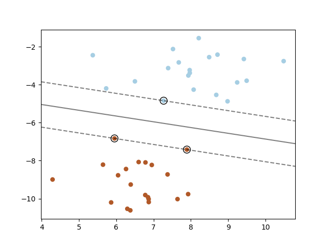
Fig. 4 A SVM aims at finding an optimal hyperplane to separate two classes in high-dimensional space, while maximizing the margin. Image from the scikit-learn SVM documentation under BSD 3-Clause license.#

We are going to train a support vector machine (SVM) classifier for brain decoding on the Haxby dataset. SVM is often successful in high dimensional spaces, and it is a popular technique in neuroimaging.

In the SVM algorithm, we plot each data item as a point in N-dimensional space where N depends on the number of features that distinctly classify the data points (e.g. when the number of features is 3 the hyperplane becomes a two-dimensional plane.). The objective here is finding a hyperplane (decision boundaries that help classify the data points) with the maximum margin (i.e the maximum distance between data points of both classes). Data points falling on either side of the hyperplane can be attributed to different classes.

The scikit-learn documentation contains a detailed description of different variants of SVM, as well as example of applications with simple datasets.

Getting the data#

We are going to download the dataset from Haxby and colleagues (2001) [HGF+01]. You can check section An overview of the Haxby dataset for more details on that dataset. Here we are going to quickly download it, and prepare it for machine learning applications with a set of predictive variable, the brain time series X, and a dependent variable, the annotation on cognition y.

import os
import warnings
warnings.filterwarnings(action='ignore')

from nilearn import datasets
# We are fetching the data for subject 4
data_dir = os.path.join('..', 'data')
sub_no = 4
haxby_dataset = datasets.fetch_haxby(subjects=[sub_no], fetch_stimuli=True, data_dir=data_dir)
func_file = haxby_dataset.func[0]

# mask the data
from nilearn.maskers import NiftiMasker
mask_filename = haxby_dataset.mask_vt[0]
masker = NiftiMasker(mask_img=mask_filename, standardize=True, detrend=True)
X = masker.fit_transform(func_file)

# cognitive annotations
import pandas as pd
behavioral = pd.read_csv(haxby_dataset.session_target[0], delimiter=' ')
y = behavioral['labels']

Let’s check the size of X and y:

categories = y.unique()
print(categories)
print(y.shape)
print(X.shape)
['rest' 'face' 'chair' 'scissors' 'shoe' 'scrambledpix' 'house' 'cat'
 'bottle']
(1452,)
(1452, 675)

So we have 1452 time points, with one cognitive annotations each, and for each time point we have recordings of fMRI activity across 675 voxels. We can also see that the cognitive annotations span 9 different categories.

Training a model#

We are going to start by splitting our dataset between train and test. We will keep 20% of the time points as test, and then set up a 10 fold cross validation for training/validation.

from sklearn.model_selection import train_test_split
X_train, X_test, y_train, y_test = train_test_split(X, y, test_size=0.2, random_state=0)   

Now we can initialize a SVM classifier, and train it:

from sklearn.svm import SVC
model_svm = SVC(random_state=0, kernel='linear', C=1)
model_svm.fit(X_train, y_train)
SVC(C=1, kernel='linear', random_state=0)
In a Jupyter environment, please rerun this cell to show the HTML representation or trust the notebook.
On GitHub, the HTML representation is unable to render, please try loading this page with nbviewer.org.

Assessing performance#

Let’s check the accuracy of the prediction on the training set:

from sklearn.metrics import classification_report
y_train_pred = model_svm.predict(X_train)
print(classification_report(y_train, y_train_pred))
              precision    recall  f1-score   support

      bottle       1.00      1.00      1.00        85
         cat       1.00      1.00      1.00        88
       chair       1.00      1.00      1.00        90
        face       1.00      1.00      1.00        81
       house       1.00      1.00      1.00        91
        rest       1.00      1.00      1.00       471
    scissors       1.00      1.00      1.00        81
scrambledpix       1.00      1.00      1.00        90
        shoe       1.00      1.00      1.00        84

    accuracy                           1.00      1161
   macro avg       1.00      1.00      1.00      1161
weighted avg       1.00      1.00      1.00      1161

This is dangerously high. Let’s check on the test set:

y_test_pred = model_svm.predict(X_test)
print(classification_report(y_test, y_test_pred))
              precision    recall  f1-score   support

      bottle       0.72      0.78      0.75        23
         cat       0.70      0.70      0.70        20
       chair       0.74      0.78      0.76        18
        face       0.89      0.93      0.91        27
       house       0.93      0.82      0.88        17
        rest       0.91      0.89      0.90       117
    scissors       0.84      0.78      0.81        27
scrambledpix       0.85      0.94      0.89        18
        shoe       0.72      0.75      0.73        24

    accuracy                           0.84       291
   macro avg       0.81      0.82      0.81       291
weighted avg       0.84      0.84      0.84       291

We can have a look at the confusion matrix:

# confusion matrix
import sys
import numpy as np
from sklearn.metrics import confusion_matrix
sys.path.append('../src')
import visualization
cm_svm = confusion_matrix(y_test, y_test_pred)
model_conf_matrix = cm_svm.astype('float') / cm_svm.sum(axis=1)[:, np.newaxis]

visualization.conf_matrix(model_conf_matrix,
                          categories,
                          title='SVM decoding results on Haxby')
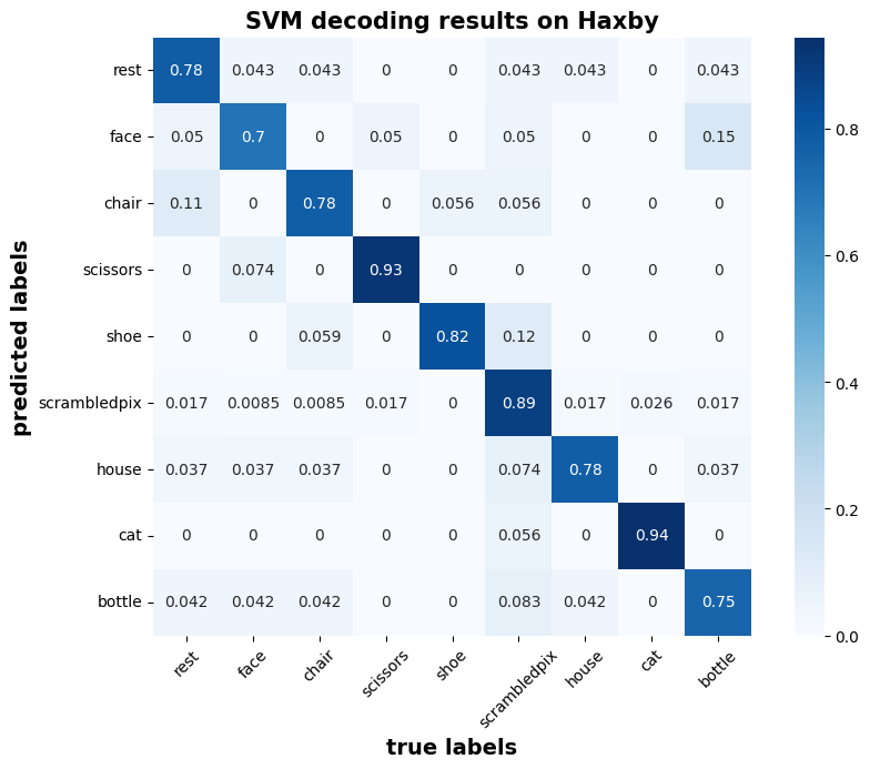
_images/2021c085709559df545bf08eb2ee051f9098c2f5619e666dceeb879ff1801dfb.png

Visualizing the weights#

Finally we can visualize the weights of the (linear) classifier to see which brain region seem to impact most the decision, for example for faces:

from nilearn import plotting
# first row of coef_ is comparing the first pair of class labels
# with 9 classes, there are 9 * 8 / 2 distinct
coef_img = masker.inverse_transform(model_svm.coef_[0, :])
plotting.view_img(
    coef_img, bg_img=haxby_dataset.anat[0],
    title="SVM weights", dim=-1, resampling_interpolation='nearest'
)

And now the easy way#

We can use the high-level Decoder object from Nilearn. See Decoder object for details. It reduces model specification and fit to two lines of code:

from nilearn.decoding import Decoder
# Specify the classifier to the decoder object.
# With the decoder we can input the masker directly.
#
# cv=5 means that we use 5-fold cross-validation
#
# As a scoring scheme, one can use f1, accuracy or ROC-AUC
#
decoder = Decoder(estimator='svc', cv=5, mask=mask_filename, scoring='f1') 
decoder.fit(func_file, y)

That’s it ! We can now look at the results: F1 score and coefficient image:

print('F1 scores')
for category in categories:
    print(f"{category.ljust(15)}    {np.mean(decoder.cv_scores_[category]):.2f}")
plotting.view_img(
    decoder.coef_img_['face'], bg_img=haxby_dataset.anat[0],
    title="SVM weights for face", dim=-1, resampling_interpolation='nearest'
)
F1 scores
rest               0.80
face               0.30
chair              0.27
scissors           0.25
shoe               0.23
scrambledpix       0.31
house              0.29
cat                0.22
bottle             0.19

Note: the Decoder implements a one-vs-all strategy. Note that this is a better choice in general than one-vs-one.

Generating sharper weight maps with L1 regularization#

Nilearn offers different flavours of SVCs. While the default uses L2 regularization under the hood, we can can obtain sharper weight maps by encouraging sparsity with L1 regularization.

_images/regularizations.png

Fig. 5 L1 penalty promotes sparsity of the estimated coefficients, while L2 penalty promotes weight sharing among all components. One can combine both L1 and L2 regularization to obtain the ElasticNet penalty.#

# Let's swap the estimator with the svc_l1
l1_decoder = Decoder(estimator='svc_l1', cv=5, mask=mask_filename, scoring='f1') 
l1_decoder.fit(func_file, y)
plotting.view_img(
    l1_decoder.coef_img_['face'], bg_img=haxby_dataset.anat[0],
    title="L1-SVM weights for face", dim=-1, resampling_interpolation='nearest'
)

We can observe that far fewer components are selected and the information is much more localized.

Getting more meaningful weight maps with Frem#

It is often tempting to interpret regions with high weights as ‘important’ for the prediction task. However, there is no statistical guarantee on these maps. Moreover, they often do not even exhibit very clear structure. To improve that, a regularization can be brought by using the so-called Fast Regularized Ensembles of models (FREM), that rely on simple averaging and clustering tools to provide smoother maps, yet with minimal computational overhead.

from nilearn.decoding import FREMClassifier
frem = FREMClassifier(estimator='svc', cv=5, mask=mask_filename, scoring='f1')
frem.fit(func_file, y)
plotting.view_img(
    frem.coef_img_['face'], bg_img=haxby_dataset.anat[0],
    title="SVM weights for face", dim=-1, resampling_interpolation='nearest'
)

Note that the resulting accuracy is in general slightly higher:

print('F1 scores with FREM')
for category in categories:
    print(f"{category.ljust(15)}    {np.mean(frem.cv_scores_[category]):.2f}")
F1 scores with FREM
rest               0.80
face               0.79
chair              0.29
scissors           0.38
shoe               0.23
scrambledpix       0.53
house              0.77
cat                0.43
bottle             0.29

⚡️ (Experimental) Running a surfacic analysis#

Nilearn recently expanded its surface API to enable surface-based decoding. We start by projecting our data onto the FreeSurfer fsaverage4 template, which is a downsampled version of the standard FreeSurfer template containing approximately 2,562 vertices per hemisphere. This template serves as the common space for analysis. We then create a SurfaceImage object that combines the mesh geometry with functional data. This object maintains separate representations for left and right hemispheres while providing a unified interface for surface-based analysis.

from nilearn.surface import vol_to_surf
from nilearn.experimental.surface._datasets import load_fsaverage
from nilearn.experimental.surface._surface_image import SurfaceImage

# We first load the fsaverage mesh
mesh = load_fsaverage("fsaverage4")["pial"]

# We then project the data on each hemisphere
data_lh = vol_to_surf(func_file, mesh["left_hemisphere"]).T
data_rh = vol_to_surf(func_file, mesh["right_hemisphere"]).T

# Then we build the SurfaceImage object
surf_img = SurfaceImage(
    mesh=mesh,
    data={
        "left_hemisphere": data_lh,
        "right_hemisphere": data_rh,
    },
)
print(f"Image shape: {surf_img.shape}")
Dataset created in /home/runner/nilearn_data/fsaverage4

Downloading data from https://osf.io/28uma/download ...
 ...done. (27 seconds, 0 min)
Extracting data from /home/runner/nilearn_data/fsaverage4/8d2777113299ca7de61b16037c37aaea/download..... done.
Image shape: (1452, 5124)

The decoder fitting process is similar to the previous ones, but with a key distinction: we implement the SurfaceMasker object for surface-based data processing. This masker is specifically designed to handle cortical surface information, allowing us to maintain the spatial structure of the brain’s surface representation throughout the decoding analysis.

# The following is just disabling a couple of checks performed by the decoder
# that would force us to use a `NiftiMasker`.
from nilearn._utils import param_validation
def monkeypatch_masker_checks():
    def adjust_screening_percentile(screening_percentile, *args, **kwargs):
        return screening_percentile

    param_validation.adjust_screening_percentile = adjust_screening_percentile
monkeypatch_masker_checks()

from nilearn.experimental.surface import SurfaceMasker

decoder = Decoder(mask=SurfaceMasker(), cv=3, screening_percentile=1)
decoder.fit(surf_img, y)

We finally plot the resulting weight map for face using an interactive surface viewer:

plotting.view_surf(
    decoder.coef_img_["face"].mesh["right_hemisphere"],
    decoder.coef_img_["face"].data["right_hemisphere"],
    cmap="coolwarm",
)

Exercises#

  • What is the most difficult category to decode? Why?

  • The model seemed to overfit. Can you find a parameter value for C in SVC such that the model does not overfit as much?

  • Try a 'rbf' kernel in SVC. Can you get a better test accuracy than with the 'linear' kernel?

  • Try to explore the weights associated with other labels.

  • Instead of doing a 5-fold cross-validation, on should split the data by runs. Implement a leave-one-run and leave-two-run out cross-validation. For that you will need to access the run information, that is stored in behavioral[chunks]. You will also need the LeavePGroupOut object of scikit-learn.

  • Try implementing a random forest or k nearest neighbor classifier.

  • Hard: implement a systematic hyper-parameter optimization using nested cross-validation. Tip: check this scikit-learn tutorial.

  • Hard: try to account for class imbalance in the dataset.